You may have heard about quantum computers and their revolutionary ability to solve computationally complex problems in an efficient manner. However, you may still not have a grasp about the fundamental concepts that make it all work together. In this series, we will go over the basic ideas underlying a quantum computer. More specifically, we will look at

• Qubits (quantum bits)
• Quantum gates and circuits
• Experimental realizations

This is part 2 in the series. If you haven't already please check out part 1.

Review

Recall that the fundamental concept of a quantum computer is the qubit and its state can be described by a quantum state of the form

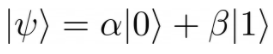
This equation tells us that the qubit can not just be in either a 0 or 1 state like a classical bit but it can also be in a superposition of 0 and 1 states. Also, the numbers alpha and beta are the probability amplitudes used to predict what the outcome of measurement will be upon squaring them. That is, when we perform a measurement, we will find the qubit to be in the state 

with probability

and in state

with probability

Performing a measurement of a qubit will change the state it is in and will cause us to lose the information about its original state.

Classical Gates

In order to implement a computation algorithm on a computer we need to use logic gates to modify the states of our bits and qubits. In a classical computer a few of the most common logic gates are AND, OR, XOR, NOT, NAND, etc. (see ref. 1). The way these logic gates work is by taking in the state of one or two bits as input and returning an output. For example the NOT gate will flip a bit from 0 to 1 and from 1 to 0. In other words

bit1 | output |

  0   |      1     |

  1   |      0     |

A two bit example takes two bits as input. For example, the AND gate will return an output of 1 if both bits are 1 and 0 otherwise. In other words we have:

bit1 | bit2 | output |

   0  |    0   |     0     |

   0  |    1   |     0     |

   1  |    0   |     0     |

   1  |    1   |     1     |

Another example is an OR gate which will return 1 if any of the bits are 1 and 0 otherwise. The table for the OR gate looks like

bit1 | bit2 | output |

   0  |    0   |     0     |

   0  |    1   |     1     |

   1  |    0   |     1     |

   1  |    1   |     1     |

By combining multiple gates across multiple bits in a computer, we can build up a circuit to perform complex algorithms. The translation of an algorithm into a circuit is not a simple task and we will not cover that here.

Quantum Gates

As you might have guessed, quantum gates come in more flavors. The two most common types of gates are the single qubit gates and the two qubit gates but there are also multi-qubit gates that are important (see ref. 2). We will only cover the first two cases. Before we begin, it is easier if we rewrite the quantum state in vector notation. This means changing the above equation for

to

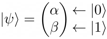
As you can see by the label on the sides, the number on top (alpha) corresponds to the probability amplitude for the state

and the number on the bottom corresponds to the probability amplitude for the state

All of the same information is contained as in the previous equation but this is a more compact form of writing it. The price we pay for this convenient notation is have to remember which number corresponds to which state.

Single qubit gates

A single qubit gate is a quantum operation we can perform on a qubit to change the state that it is in. Applying a single qubit gate will change the factors alpha and beta therefore changing the state that the qubit is in. Single qubit gates are often called rotations because, in the vector notation, changing alpha and beta is like rotating a vector. The way a single qubit gate is written is using a 2x2 matrix:

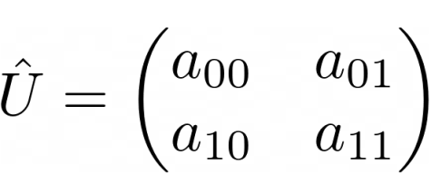
Here, the hat over the U means that U is a matrix and the a_00, a_01, a_10, a_11, are the entries of the matrix. The first number in the subscript is the row index and the second is the column index. For example a_01 means the entry in the 0th row and 1st column. Note that the counting of the index starts from 0.

In order to apply this gate to a quantum state, we just perform matrix * vector multiplication:

To understand this equation lets read it from left to right:

The first part says that we want to apply the gate U to the quantum state psi.

The second part we just replace U by its matrix representation and psi by its vector representation.

In the last part we do the matrix multiplication and get and output vector which is the new quantum state of psi.

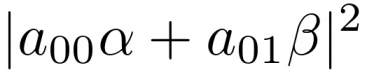
By applying the gate, we have "rotated" the original quantum state. What effect does this have? Now when we perform a measurement, we have changed the probability amplitudes and so the probability of measuring the state

is

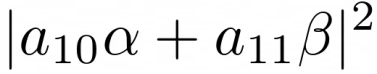
and the probability of measuring the state

is

Let's look at a more concrete example and suppose we start with a qubit in the state

and we want to know what happens when we apply an X gate. The operation we are performing is given by

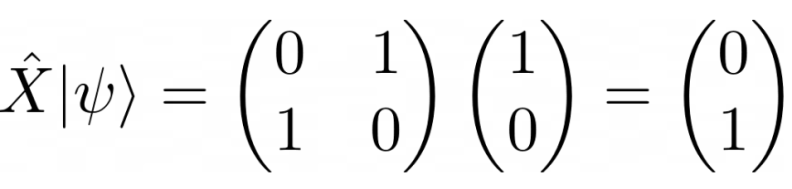
Reading this again from left to right:

The first part says we want to apply the X gate to our quantum state psi.

The X gate is given by the matrix that is written there (which we can get from ref. 2) and our initial state is only the | 0 > state.

So its vector representation is written there which has alpha = 1 and beta = 0.

The third part shows the result of doing the matrix multiplication and the new state of psi. This state has alpha = 0 and beta = 1!

By applying an X gate to our qubit we have flipped its state from 

to 

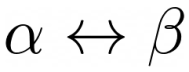
This is the quantum version of the classical NOT gate we saw before. You should verify for yourself that if you start with the | 1 > state and apply an X gate you will be flipped to the | 0 > state. You may also notice that if you try a superposition state with arbitrary values of alpha and beta, the probability amplitudes will swap

Let's look at another interesting gate called the Hadamard gate:

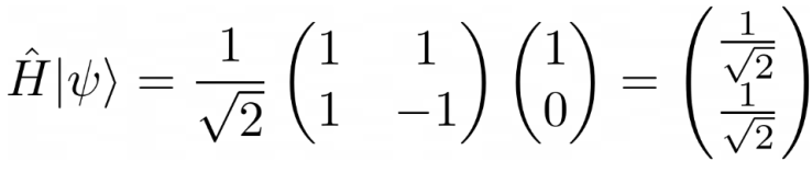
The Hadamard gate is used to create a superposition state. We started with a state that had alpha = 1 and beta = 0 but after applying the Hadamard gate we ended up with a new state that has alpha = 1/sqrt(2) and beta = 1/sqrt(2). If we were to measure the qubit before applying the Hadamard gate we would have found it to be in the state | 0 > with absolute certainty. However, after applying the Hadamard gate, if were to measure the qubit we would find it in the state | 0 > with 50% probability and | 1 > with 50% probability. In experiments, it is easier to prepare a qubit in a | 0 > or | 1> state and then use a Hadamard gate to create the superposition state rather than preparing the superposition state directly.

This article is getting longer than I expected so I've decided to split it up into multiple parts. Don't forget to follow to get a notification when the next part becomes available.