In this post we are going over the step-by-step implementation of a trading algorithm for Crypto using three technical indicators: Bollinger Bands, Relative Strength Index (RSI) and the Schaff Trend Cycle (STC).
Please note: I am not proposing any trading strategies. This post is for educational purposes only. None of the code examples have been tested. Use at your own risk. Any type of investment is inherently risky.
What is the RSI?
According to Investopedia.com, the relative strength index (RSI) is a momentum indicator used in technical analysis that measures the magnitude of recent price changes to evaluate overbought or oversold conditions in the price of a stock or other asset.
The RSI is displayed as an oscillator (a line graph that moves between two extremes) and can have a reading from 0 to 100.
The traditional interpretation of entry and exit points is that an RSI of 70 or above indicates that a security is becoming overbought or overvalued and may be destined for a trend reversal. An RSI value of 30 or below on the other hand indicates an oversold or undervalued condition.
What are Bollinger Bands?
Bollinger Bands (BB) are a volatility indicator developed by John Bollinger, a 1980’s trading technician.
BBs consist of a centerline and two price channels (bands) above and below it. The centerline is typically a simple moving average and the price channels are the standard deviations of the price examined.
When the price touches the lower band, prices are considered, oversold triggering a buy signal. Conversely, when the price touches the upper Bollinger Band, the prices are thought to be overbought triggering a sell signal.
What is the Schaff Trend Index?
The Schaff Trend Index (STC) is a trend indicator developed by Doug Schaff in 1999. The STC indicator is a forward-looking, leading indicator, that generates faster, more accurate signals than earlier indicators, such as the MACD because it considers both time (cycles) and moving averages.
The STC indicator generates its buy signal when the signal line turns up from 25 to indicate a bullish reversal. Conversely, the STC generates a sell signal when the indicator turns down from 75.
Why use this combination of indicators?
I chose this combination of technical indicators for three reasons:
-
First, they each measure different things and thus complete each other in regards to generating signals. The RSI is a momentum indicator and measure changes in stock price. Bollinger Bands are a measure of price volatility. Finally, the STC is a trend indicator used to provide a direction in which the price is moving.
-
The second reason why I used this combination is because I had recently researched which indicators are used by experts technical analysis (see my post here) and these were on the top of the list.
-
The third reason is that these indicators generate clear, measurable entry and exit signals and are thus suitable for trade automation.
The Implementation
Let’s jump into the code already. You can find a link to the full implementation as a Jupyter Notebook at the end of this post.
This section is used to import the required Python libraries. If you don’t have them installed in your environment, you will have to install them first.
from datetime import datetime
import sys
import os
import math
import numpy as np
import pandas as pd
import pandas_ta as ta
from ta.volatility import BollingerBands
from ta.volatility import KeltnerChannel
from ta.trend import STCIndicator
import datetime
from pandas.tseries.holiday import USFederalHolidayCalendar
from pandas.tseries.offsets import CustomBusinessDay
US_BUSINESS_DAY = CustomBusinessDay(calendar=USFederalHolidayCalendar())
import matplotlib.pyplot as plt
import plotly.graph_objects as go
from plotly.subplots import make_subplots
import itertools
import matplotlib.dates as mpl_dates
The next block is a helper function to load a data file with crypto prices.
You can either download the data file from here for testing or you can download crypto live data using the instructions in my recent post here.
def load_data_file(symbol):
    #  Create output file name
    daily_file_name = "{}_1d_1m.csv".format(symbol)
    daily_full_path = os.path.join('C:\\dev\\trading\\tradesystem1\\data\\crypto\\', daily_file_name)

    #  Check if output file exists
    if os.path.exists(daily_full_path):
        df = pd.read_csv(daily_full_path, parse_dates=True)
        if df.empty:
            return None
        df['Date'] = pd.to_datetime(df['Datetime'])
        df['Date'] = df['Date'].apply(mpl_dates.date2num)
        df = df[["Date", "Open", "High", "Low", "Close", "Volume"]]
        return df
    else:
        return None
The next function is used to calculate the technical indicators using the pandas-ta library for Bollinger Bands, RSI and STC.
def calculate_tis(df):
    bb_window = 20
    indicator_bb = BollingerBands(close=df['Close'], window=bb_window, window_dev=2)

    # Add Bollinger Bands features
    df['BB_mid'] = indicator_bb.bollinger_mavg()
    df['BB_high'] = indicator_bb.bollinger_hband()
    df['BB_low'] = indicator_bb.bollinger_lband()

    rsi_window = 14
    df['RSI'] = ta.rsi(df['Close'], window=rsi_window)

    stc_window_slow = 50
    stc_window_fast = 23
    stc_cycle = 10
    indicator_stc = STCIndicator(close=df['Close'], window_slow=stc_window_slow, window_fast=stc_window_fast, cycle=stc_cycle, smooth1=3, smooth2=3)

    # Add features
    df['STC'] = indicator_stc.stc()

    return df
This function is used to calculate the entry and exit signals for each technical indicator. As you can see I played around with the values a bit.
For the Bollinger Bands I added an adjusted lower and upper band that is based on a percentage of the price range during that period. The intention here was to optimize the strategy results.
def calculate_signals(df):
    df['RSI_entry_ind'] = np.where(np.logical_and((df['RSI'] > 34), (df['RSI'].shift() <= 34)), 1, 0)
    df['RSI_exit_ind'] = np.where(np.logical_and((df['RSI'] < 84), (df['RSI'].shift() >= 84)), 1, 0)

    #  Calculate upper / lower boundary for BB
    close_prices = df['Close'].to_numpy()
    max_close = np.amax(close_prices)
    min_close = np.amin(close_prices)
    diff_close = max_close - min_close
    df['BB_low_adj'] = df["BB_low"] + (diff_close * 0.09)
    df['BB_entry_ind'] = np.where((df["Close"] <= df["BB_low_adj"]), 1, 0)
    df['BB_high_adj'] = df["BB_high"] - (diff_close * 0.07)
    df['BB_exit_ind'] = np.where((df["Close"] >= df["BB_high_adj"]), 1, 0)

    df['STC_entry_ind'] = np.where(np.logical_and(df['STC'] > 73, df['STC'].shift() <= 73), 1, 0)
    df['STC_exit_ind'] = np.where(np.logical_and(df['STC'] < 97, df['STC'].shift() >= 97), 1, 0)
    return df
This function executes the strategy by iterating through the actual crypto price and checking for entry and exit signals.
As you can see I’m also using a lookback period of 20 time periods. The reason for this is that the entry and exit signals likely don’t occur at exactly the same time. Instead, the may occur in sequence, e.g. BB - STC - RSI.
That’s why from every time period, we are looking back 20 periods to see if all the signals fired during that lookback period.
def execute_strategy(df):
    close_prices = df['Close'].to_numpy()
    rsi_entry = df['RSI_entry_ind'].to_numpy()
    rsi_exit = df['RSI_exit_ind'].to_numpy()
    bb_entry = df['BB_entry_ind'].to_numpy()
    bb_exit = df['BB_exit_ind'].to_numpy()
    stc_entry = df['STC_entry_ind'].to_numpy()
    stc_exit = df['STC_exit_ind'].to_numpy()

    required_entry_signals = 3
    required_exit_signals = 3

    last_entry_price = 0
    entry_prices = []
    exit_prices = []
    hold = 0

    for i in range(len(close_prices)):
        current_price = close_prices[i]
        num_entry_signals = 0
        num_exit_signals = 0

        lookback_ind = i - 20
        if lookback_ind >= 0:
            rsi_entry_lookback = rsi_entry[lookback_ind:i]
            if 1 in rsi_entry_lookback:
                num_entry_signals += 1
            rsi_exit_lookback = rsi_exit[lookback_ind:i]
            if 1 in rsi_exit_lookback:
                num_exit_signals += 1

            bb_entry_lookback = bb_entry[lookback_ind:i]
            if 1 in bb_entry_lookback:
                num_entry_signals += 1
            bb_exit_lookback = bb_exit[lookback_ind:i]
            if 1 in bb_exit_lookback:
                num_exit_signals += 1

            stc_entry_lookback = stc_entry[lookback_ind:i]
            if 1 in stc_entry_lookback:
                num_entry_signals += 1
            stc_exit_lookback = stc_exit[lookback_ind:i]
            if 1 in stc_exit_lookback:
                num_exit_signals += 1

        #  Verify Entry indicators
        if hold == 0 and num_entry_signals >= required_entry_signals:
            last_entry_price = current_price
            entry_prices.append(current_price)
            exit_prices.append(np.nan)
            hold = 1
        #  Exit strategy
        elif hold == 1 and num_exit_signals >= required_exit_signals:
            entry_prices.append(np.nan)
            exit_prices.append(current_price)
            hold = 0
        else:
            #  Neither entry nor exit
            entry_prices.append(np.nan)
            exit_prices.append(np.nan)

    return entry_prices, exit_prices
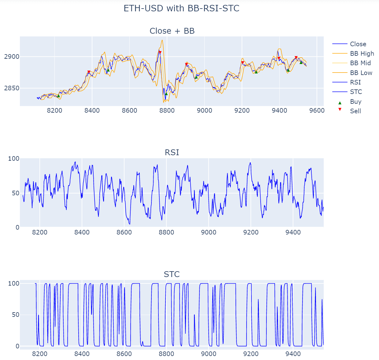
This next function is used to visualize the results by plotting the price graph along with the BBs, and below in separate graphs the RSI and STC.
def plot_graph(symbol, df, entry_prices, exit_prices):
    fig = make_subplots(rows=3, cols=1, subplot_titles=['Close + BB','RSI','STC'])

    #  Plot close price
    fig.add_trace(go.Line(x = df.index, y = df['Close'], line=dict(color="blue", width=1), name="Close"), row = 1, col = 1)

    #  Plot bollinger bands
    bb_high = df['BB_high']
    bb_mid = df['BB_mid']
    bb_low = df['BB_low']
    fig.add_trace(go.Line(x = df.index, y = bb_high, line=dict(color="orange", width=1), name="BB High"), row = 1, col = 1)
    fig.add_trace(go.Line(x = df.index, y = bb_mid, line=dict(color="#ffd866", width=1), name="BB Mid"), row = 1, col = 1)
    fig.add_trace(go.Line(x = df.index, y = bb_low, line=dict(color="orange", width=1), name="BB Low"), row = 1, col = 1)

    #  Plot RSI
    fig.add_trace(go.Line(x = df.index, y = df['RSI'], line=dict(color="blue", width=1), name="RSI"), row = 2, col = 1)

    #  Plot STC
    fig.add_trace(go.Line(x = df.index, y = df['STC'], line=dict(color="blue", width=1), name="STC"), row = 3, col = 1)

    #  Add buy and sell indicators
    fig.add_trace(go.Scatter(x=df.index, y=entry_prices, marker_symbol="arrow-up", marker=dict(
        color='green',
    ),mode='markers',name='Buy'))
    fig.add_trace(go.Scatter(x=df.index, y=exit_prices, marker_symbol="arrow-down", marker=dict(
        color='red'
    ),mode='markers',name='Sell'))

    fig.update_layout(
        title={'text':f"{symbol} with BB-RSI-STC", 'x':0.5},
        autosize=False,
        width=800,height=800)
    fig.update_yaxes(range=[0,1000000000],secondary_y=True)
    fig.update_yaxes(visible=False, secondary_y=True)  #hide range slider

    fig.show()
Next is a function used to calculate the profit based on an initial investment and the sets of entry and exit prices we generated from executing the strategy.
def calculate_profit(start_investment, entry_prices, exit_prices):
    hold = 0
    profit = 0
    available_funds = start_investment
    cost = 0
    num_stocks = 0
    for i in range(len(entry_prices)):
        current_entry_price = entry_prices[i]
        current_exit_price = exit_prices[i]

        if not math.isnan(current_entry_price) and hold == 0:
            num_stocks = available_funds / current_entry_price
            cost = num_stocks * current_entry_price
            hold = 1

        elif hold == 1 and not math.isnan(current_exit_price):
            hold = 0
            proceeds = num_stocks * current_exit_price
            profit += proceeds - cost

    return math.trunc(profit)
Finally, we have the main() function that executes all the other functions in sequence.
Here we are using the price data for the Cryptocurrency ‘Ethereum’, a start investment of $1,000 and we are only using 1440 time periods, so about 24 hours of data.
# MAIN
symbol = 'ETH-USD'
start_investment = 1000
df = load_data_file(symbol)
df = df.tail(1440)
df = calculate_tis(df)
df = calculate_signals(df)

entry_prices, exit_prices = execute_strategy(df)
profit = calculate_profit(start_investment, entry_prices, exit_prices)
trades = np.array(exit_prices)
num_trades = len(trades[~np.isnan(trades)])
print(f"Number of trades: {num_trades}")
print(f"Profit with start_investment of ${start_investment}: ${profit}")
plot_graph(symbol, df, entry_prices, exit_prices)
Results
Here the output of this python:
Number of trades: 6
Profit with start investment of $1000: $51
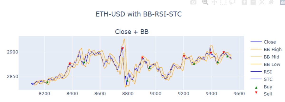
As you can see from the graph below, we are nicely setting the entry points (green arrow up) and the exit points (red arrow down) of this strategy in the peaks and valleys of the curve. The combination of the indicators seems to have done a good job of providing accurate signals.
It is also apparent, that the strategy does well following along with long upwards trends as you can see in the periods between 8500 and 8800.
However, the strategy doesn’t see to do well with sudden downturns are you can see after the entry point around period 9000.
In regards to profitability, the strategy seems to do well for this case. It generated a $51 profit in a 24-hour period with a $1,000 investment (if my code is correct). That’s a 5.1% return - sweet!
Next Steps
So now that we implemented a strategy that seems worth pursuing here are some of the next steps:
-
Backtesting, backtesting, backtesting with historic data of other crypto coins to make sure the strategy didn’t just work well for this one case. Also consider running this strategy against longer periods of data.
-
Consider implementing a stop loss guard to protect from sudden market turndowns.
-
Consider implementing a trailing stop loss to protect your gains.
-
More backtesting.
Wrapping up
In this post we examined a combination strategy using three technical indicators: Bollinger Bands, RSI and STC. We also discussed the reasons why I chose them. In the second part we went over the Python implementation of this strategy and in the last section we reviewed the results and discussed next steps.
You can find a complete implementation of this strategy on my GitHub repo here.
I hope this post provided some value for you.
Happy trading!