As I alluded to in my previous post, our implementation to our DBSCAN algorithm has a few shortcommings. So I want to take the time to go through the thought process of taking an algorithm we wrote and improving it to get better results. I probably won't make much posts like this as I usually do this behind the scenes. But I thought it would be educational to try to elaborate on how I tweak functions to make the more dynamic and adaptable when it comes to adjusting them to financial data. The most important of all is the fact that this code doesn't take into account the differences in scale when defining the eps parameter. To address this is simple, we will replace our eps parameter with an eps_percentage parameter and instead of compare the distances with an absolute value we shall compare them with a percentage of the average price of our data.

def dbscan(prices, eps_percent=0.005%, min_samples=5):
    #initialization
    clusters = []
    #we will use sets for visited and noise to make sure they are unique
    visited = set()
    noise = set()
    
    #initialize the eps value as a portion of the mean
    eps = (sum(prices) / len(prices)) * eps_percent
    

So for now we will be using 0.5% of the average price of our data as the threshold for neighboring points. Let's take a look at the results. I will be using 1D intervals of the past 6 months for the ETH/USD pair. What we should get in return is a tuple of lists. One is a list of lists, each representing a cluster. The other is a lost of indexes representing the noise.

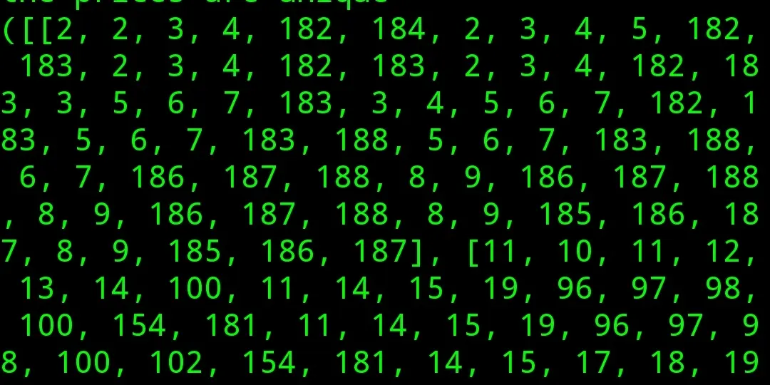
This output looks crazy but let's clean it up a bit. Let's make a function that helps us find liquidity with our DBSCAN function. So the following would be a cleanup of the clusters so that only unique points are in each cluster. Since we added all neighbors we will convert each cluster to a set and then back into a list with a list comprehension:

def find_liquidity_dbscan(prices):
    clusters, noise = dbscan(prices)
    
    clusters = [list(set(c)) for c in clusters]
    print(len(clusters))
    for cluster in clusters:
        print(cluster)

So let's take a look at our cleaned up output:

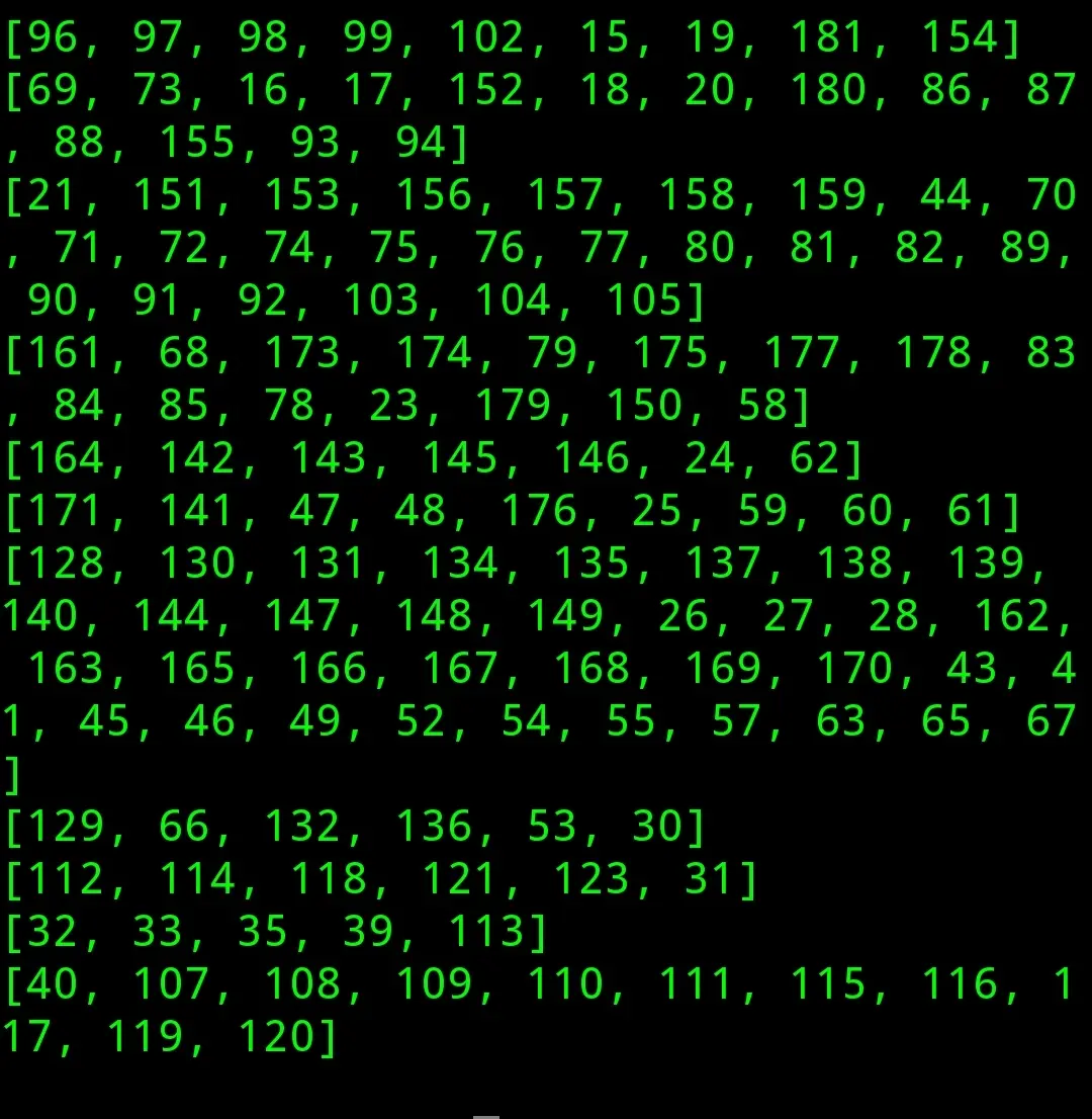
So as we can see we have 11 clusters, each containing the indexes of the periods where prices closed withing 0.05% of eachother. So now let's use our price list to extract the timestamps and closing prices to see how this looks:

def find_liquidity_dbscan(prices):
    clusters, noise = dbscan([x["closing"] for x in prices])
    
    clusters = [list(set(c)) for c in clusters]
    
    print(f"{len(clusters)} clusters found.")
    
    cluster_data = []
    
    for cluster in clusters:
        data = [{ "timestamp": prices[c]["timestamp"], "price": prices[c]["closing"]} for c in cluster]
        
        cluster_data.append(data)
        
    print(cluster_data[0])

As you can see in the last line of that function we are going to isolate the first cluster to see how it looks like. Let's view our output:

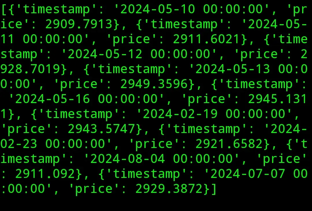
We can see that the prices are relatively close to eachother but not enough in my opinion. The new problem we are up against is the fact that obviously different price ranges have different sensitivity to the percentage we use. If it's price is in the thousands small percentages will lead to bigger absolute prices, and if a coin's price is fractions of cents then we will need bigger percentages to detect significant variations in price. I stumbled into a similar problem with try to automate the detection of price action patterns. For example in the head and shoulders pattern I wanted to make sure that the shoulders where at approximately the same height. The solution to this dilemma was using the ATR indicator. I wont go into much detail but it indicates the volatility a price has locally. Doesn't matter the direction as if you see in the formula it uses absolute values. Since I don't want to go much on a tangent I will use my ATR function that takes a lost of dictionaries with ohlc price data and returns a list of dictionaries with timestamps and ATR values:

def tr(prices):
    """
    calculate the true range
    """
    
    trs = []
    
    for i in range(1, len(prices)):
        high = prices[i]["highest"]
        low = prices[i]["lowest"]
        prev = prices[i - 1]["closing"]
        
        tr = max(high - low, abs(prev - low), abs(prev - high))
        
        data = {
            "timestamp": prices[i]["timestamp"],
            "tr": tr
        }
        
        trs.append(data)
        
    return trs
    
def atr(prices, periods=14):
    """
    calculate atr over periods smoothed with rma
    """
    trs = tr(prices)
    
    atrs = rma(trs, periods, "tr", "atr")
    
    atrs = [{"timestamp": prices[0]["timestamp"], "atr": None}] + atrs
    
    return atrs

For readability I separated this code into two functions. One that calculates the true range and another one that calculates the average true range. I also like to be extra fancy so as you can see i added rma smoothing. If you want to do that too here is my function:

def rma(values, periods, source, result):
    """
    The running moving average
    used for smoothing lines like ATR
    """
    rmas = [{"timestamp": value["timestamp"], result: None} for value in values]
    
    initial = sum(value[source] for value in values)
    
    if(len(values) >= periods):
        rmas[periods - 1][result] = initial / periods
        
        for i in range(periods, len(values)):
            prev = rmas[i - 1][result]
            
            rma = (prev * (periods - 1) + values[i][source]) / periods
            
            rmas[i][result] = round(rma, 4)
            
    return rmas   

I added a little doc string for people who aren't familiar with the  RMA indicator. So to make our eps relative to price and volatility and not dependant on any hardcoded value, we will take the average of the ATR and get a percentage of it and use that as our eps value. So the initialization of our eps would look like:

#use the average atr to make eps dynamic
    atrs = [a["atr"] for a in atrs if a["atr"]]
    eps = (sum(atrs) / len(atrs)) * .05

After a bit of trial and error I found that using 5% of it gives us some nice and satisfactory answers. Here are my results:

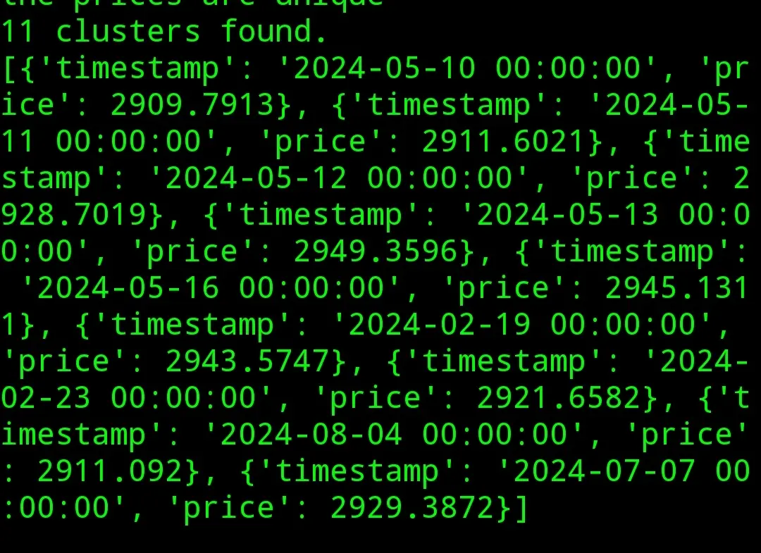
So as we can see, we can prices that are closer together. Now remember these aren't liquidity zones per se, they are prices where a significant amount of trades have occurred. So let's clean it up by going through each cluster, averaging the prices and registering the timestamps for these prices:

def find_liquidity_dbscan(prices):
    atrs = atr(prices)
    clusters, noise = dbscan([x["closing"] for x in prices], atrs)
    
    clusters = [list(set(c)) for c in clusters]
    
    print(f"{len(clusters)} clusters found.")
    
    cluster_data = []
    
    for cluster in clusters:
        data = [{ "timestamp": prices[c]["timestamp"], "price": prices[c]["closing"]} for c in cluster]
        
        avg_price = sum(x["price"] for x in data) / len(data)
        timestamps = [x["timestamp"] for x in data]
        
        cluster_data.append({"zone": avg_price, "touches": timestamps})
        
    for cluster in cluster_data:
        print(f"high activity price: {cluster['zone']}")
        print(f"times touched: {len(cluster['touches'])}")
        
        for timestamp in cluster["touches"]:
            print(f"->{timestamp}")
        

In the results I found something quite interesting:

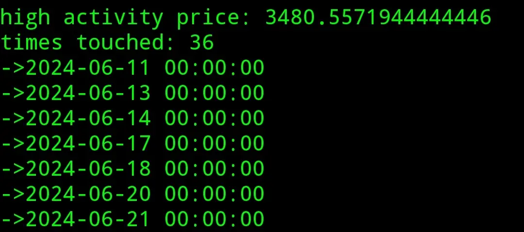
So we can see for ETHUSD the price closed around 3840 36 times in the last approximately 180 days. So we can automatically predict that price action usually reacts around this price zone.

I'm going to leave it here and work on the next article which will be another clustering algorithm so stay tuned. 

You can follow me on Twitter to get updates on my future posts and also some signals that are generated by other strategies.