Hi,

My name is Michael, I'm a physics graduate and now work as a software engineer. As I'm new to Bitcoin I thought it would be a good idea to do some exploratory data analysis using Pandas. This will be a beginner's guide to using Pandas, with this first part showing you how to:

• Read historical Bitcoin data from a CSV into a Pandas dataframe.
• Create a time series of these data.
• Plot the price of Bitcoin over its entire history.

Once this is done, we'll look at what else Pandas has to offer, but for now, this will be a good starting point. I'll show everything step-by-step, the only assumption I'll make is that you have python installed and you are a little familiar with using it. Code that goes into your script will be in bold below.

Let's get started!

1. The first thing we need is the historical price data of Bitcoin, which is easily found with a quick google search. I visited CryptoDataDownload.com 

and used the Coinbase exchange to get the daily historical prices for Bitcoin. Save this as a comma-separated value (CSV) file and open up whatever you normally use to create and edit Python scripts. I will be using PyCharm, one of the best Integrated Development Environments (IDE) I've ever come across, which you can download the Community Edition for free from their website https://www.jetbrains.com/pycharm/.

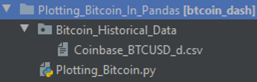
Create a new script with a sensible name (I choose Plotting_Bitcoin.py) and in the same directory create another directory (Bitcoin_Historical_Data) to hold the historical price data, and put the CSV file in this directory:

The first part of the script will import the necessary libraries, which are classes and functions written by other programmers that we can use:

# Import libraries
import pandas as pd
import matplotlib.pyplot as plt
import os

If you're not familiar with Python, comments start with the hash character, #, and extend to the end of the physical line. I'll be using comments to add little notes throughout the program to say what is happening.

2. Now we need to read in our CSV data into a Pandas dataframe, and we can use the Pandas function:

pd.read_csv("CSV_File_Path_Location")

When giving the path location, you can provide a full file path e.g. "C:/SomeFolder/SomeFile.ext", or alternatively, if you just list a file name, e.g. pd.read_csv("Coinbase_BTCUSD_d.csv") python will look in the current working directory for that file.

If it isn't found, Python will throw a FileNotFound Error. We'll use the second means, and provide a path relative to the current working directory by creating a path using the folder name and file name:

# Folder name of the directory where the data is stored
folder_name = 'Bitcoin_Historical_Data'

# Name of the csv file to load into a pandas dataframe
btc_daily = 'Coinbase_BTCUSD_d.csv'

# Join various path components
btc_daily_path = os.path.join(folder_name, btc_daily)

Here I used the function os.path.join() to intelligently join my path components by automatically using the correct system separator (\ vs /). If we run this program and inspect the variable btc_daily_path we see:

btc_daily_path = 'Bitcoin_Historical_Data\\Coinbase_BTCUSD_d.csv'

We can now use this to create our historic prices dataframe:

# Read in csv file data into pandas dataframe
btc_daily_df = pd.read_csv(btc_daily_path)

You can think of a dataframe exactly like an excel spreadsheet, with a height in rows, and width in columns. We can look at the top part of our dataframe using the .head(n) function, which will show you the top n rows of your dataframe, with column names appearing at the top and a row index on the left:

# Look at the top seven rows of the dataframe
print(btc_daily_df.head(7))

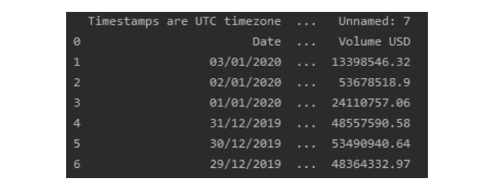
Whoops, looking at the first column name 'Timestamps are UTC timezone', I clearly forgot that the first row of the CSV file contains
comments. we'll use the 'skiprows' parameter in read_csv to skip that first row:

# Read in csv file data into pandas dataframe
btc_daily_df = pd.read_csv(btc_daily_path, skiprows=1)

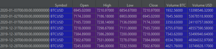
Now, if we look at the top seven rows again (I'll use PyCharm to display it this time as it looks better this way):

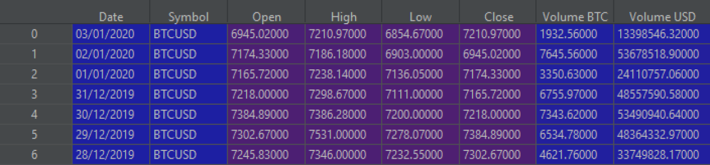
Great, we now have our historical Bitcoin prices in a dataframe, with the correct column headings. Let's have a quick inspection of this
dataframe with some other useful Pandas functions:

# Look at the bottom 3 rows of the dataframe
print(btc_daily_df.tail(3))

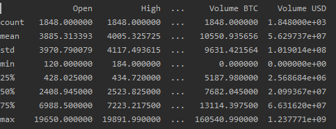
# Get some quick statistics on the dataframe
print(btc_daily_df.describe())

# Look at the format of the columns
print(btc_daily_df.info())

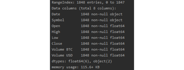
We can see we have 8 columns in total, with 1848 rows, and we are not missing any data from any columns as all 1848 rows are non-null. If
you take a look at the CSV, you'll see that the Date and Symbol columns are actually strings, and the remaining columns have been recognised
as floats.

An extremely useful feature of Pandas is the ability to operate on a dataframe with an index that consists of dates and/or times. To do
this, we will first transform the 'Date' column into a datetime series:

# Convert the 'Date' column to datetime format
btc_daily_df['Date'] = pd.to_datetime(btc_daily_df['Date'], format='%d/%m/%Y')

Taking a look at the column types again:

# Look at the format of the columns
print(btc_daily_df.info())

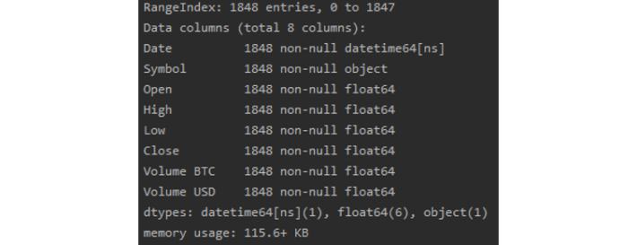
We see that the 'Date' column is now of the datatime64[ns] type. Now, we can set the 'Date' column as an index:

# Set the 'Date' Column as the index
btc_daily_df = btc_daily_df.set_index('Date')

Finally, we can use this dataframe to plot our data. The next bit of code plots the 'Open' prices against the index column, and sets a
couple of the plot parameters. It also saves the plot image in the same directory as the CSV file:

# Plot the Bitcoin open prices
btc_daily_df.plot(y='Open',
title='Bitcoin Opening Prices',
grid=True,
color='blue',
)
# the plot gets saved to 'BTC_USD_daily_plot.png'
save_path = os.path.join(folder_name, 'BTC_USD_daily_plot.png')
plt.savefig(save_path)
plt.show()

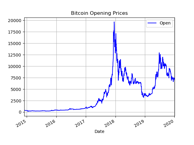
With only a few lines of code, we were able to produce a nice looking plot of the historic Bitcoin opening prices.

I hope you've enjoyed this beginner's guide to using Pandas for Bitcoin data analysis, and I'll see you In my next post, where we will
delve deeper into the Pandas timeseries operations and see what kind of information we can glean from the data.